885. Spiral Matrix III

You start at the cell (rStart, cStart) of an rows x cols grid facing east. The northwest corner is at the first row and column in the grid, and the southeast corner is at the last row and column.

You will walk in a clockwise spiral shape to visit every position in this grid. Whenever you move outside the grid’s boundary, we continue our walk outside the grid (but may return to the grid boundary later.). Eventually, we reach all rows * cols spaces of the grid.

Return an array of coordinates representing the positions of the grid in the order you visited them.

Example 1:

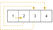
Input: rows = 1, cols = 4, rStart = 0, cStart = 0
Output: [[0,0],[0,1],[0,2],[0,3]]

Example 2:

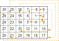
Input: rows = 5, cols = 6, rStart = 1, cStart = 4
Output: [[1,4],[1,5],[2,5],[2,4],[2,3],[1,3],[0,3],[0,4],[0,5],[3,5],[3,4],[3,3],[3,2],[2,2],[1,2],[0,2],[4,5],[4,4],[4,3],[4,2],[4,1],[3,1],[2,1],[1,1],[0,1],[4,0],[3,0],[2,0],[1,0],[0,0]]

Constraints:

• 1 <= rows, cols <= 100
• 0 <= rStart < rows
• 0 <= cStart < cols

Approach 01:

#include <vector>

using namespace std;

class Solution {
 public:
  vector<vector<int>> spiralMatrixIII(int numRows, int numCols, int startRow, int startCol) {
    // Direction vectors: right, down, left, up
    const vector<int> xDirections{1, 0, -1, 0};
    const vector<int> yDirections{0, 1, 0, -1};
    
    // Resultant matrix with the starting point
    vector<vector<int>> result{{startRow, startCol}};

    // Loop until we fill the matrix
    for (int i = 0; result.size() < numRows * numCols; ++i) {
      for (int step = 0; step < i / 2 + 1; ++step) {
        // Move in the current direction
        startRow += yDirections[i % 4];
        startCol += xDirections[i % 4];
        
        // Check if the new position is within the bounds
        if (0 <= startRow && startRow < numRows && 0 <= startCol && startCol < numCols) {
          result.push_back({startRow, startCol});
        }
      }
    }

    return result;
  }
};

class Solution:
    def spiralMatrixIII(self, numRows: int, numCols: int, startRow: int, startCol: int) -> List[List[int]]:
        # Direction vectors: right, down, left, up
        xDirections = [1, 0, -1, 0]
        yDirections = [0, 1, 0, -1]
        
        # Resultant matrix with the starting point
        result = [[startRow, startCol]]
        
        # Loop until we fill the matrix
        i = 0
        while len(result) < numRows * numCols:
            for step in range(i // 2 + 1):
                # Move in the current direction
                startRow += yDirections[i % 4]
                startCol += xDirections[i % 4]
                
                # Check if the new position is within the bounds
                if 0 <= startRow < numRows and 0 <= startCol < numCols:
                    result.append([startRow, startCol])
            i += 1
        
        return result

Time Complexity

• Matrix Traversal:

  The algorithm traverses each cell of the matrix exactly once, and for each step, it checks if the current position is within the matrix bounds. Therefore, the time complexity is \( O(n \times m) \), where \( n \) is the number of rows and \( m \) is the number of columns in the matrix.

Space Complexity

• Resultant Matrix:

  The space complexity is dominated by the storage required for the resultant matrix, which contains all the positions in the matrix. Since the result vector stores all \( n \times m \) positions, the space complexity is \( O(n \times m) \).

• Additional Space:

  The algorithm uses a constant amount of extra space for variables such as direction vectors and loop counters. Therefore, the additional space complexity is \( O(1) \).

• Overall Space Complexity:

  Considering both the resultant matrix and the additional space, the overall space complexity is \( O(n \times m) \).